AVL Tree vs. Binary Search Tree (BST) Visualizer
When learning data structures, the difference between an ordinary Binary Search Tree (BST) and an AVL Tree often seems purely theoretical until you actually try to insert sequential data.
When learning data structures, the difference between an ordinary Binary Search Tree (BST) and an AVL Tree often seems purely theoretical until you actually try to insert sequential data. A standard BST is easy to implement, but it harbors a fatal flaw that an AVL tree is specifically designed to fix.
By using an interactive tree simulator, you can visualize exactly why self-balancing algorithms are necessary for modern database indexing and high-performance search applications.
The Fatal Flaw of the Standard BST
A standard Binary Search Tree operates on a simple rule: values smaller than the current node go to the left; values larger go to the right.
If you insert random, unsorted data (e.g., 50, 20, 80, 10, 30), the tree naturally branches out. Searching for any value in a nicely branched tree takes $O(\log n)$ time.
But what happens if you insert sorted data?
Open a BST simulator and try inserting the numbers 10, 20, 30, 40, 50 in that exact order.
Because every new number is larger than the last, the tree never branches to the left. It simply creates a long line pointing down and to the right. The tree has structurally degraded into a linked list.
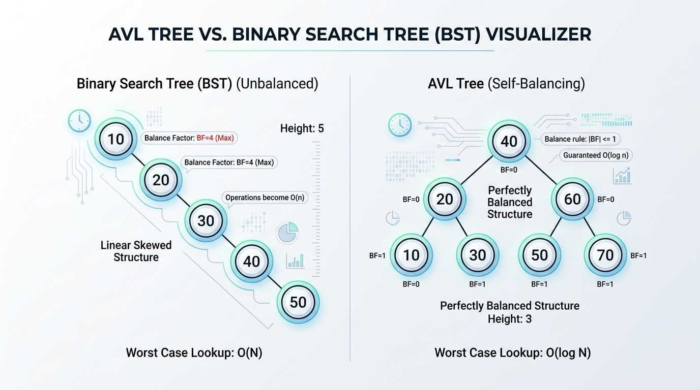
If you have 10,000 sorted records and search for the last one in a standard BST, the algorithm has to check all 10,000 nodes. Your $O(\log n)$ search time has catastrophically degraded to $O(n)$ time.
The AVL Tree Solution: Enforced Balance
An AVL tree prevents this degradation. It is a Binary Search Tree, meaning it follows the exact same left/right ordering rules, but it adds a strict constraint: the heights of the left and right subtrees of any node can never differ by more than 1.
If you take those same sorted numbers (10, 20, 30, 40, 50) and insert them into an AVL Tree Visualizer, you will see a radically different outcome.
- Insert 10. (Root node created).
- Insert 20. (Attaches to the right of 10).
- Insert 30. (Attaches to the right of 20).
At this exact moment, the AVL tree calculates the balance factor of node 10 and realizes the right side is too heavy. It immediately performs a Left Rotation, pulling 20 up to become the new root.
As you continue inserting 40 and 50, the AVL tree will continue to automatically rotate the branches, forcing the tree to stay wide and shallow rather than long and narrow.
Side-by-Side Comparison Summary
| Feature | Standard Binary Search Tree (BST) | AVL Tree |
|---|---|---|
| Insertion Logic | Simple left/right comparison. | Left/right comparison + Height updates + Rotations. |
| Best Case Search | $O(\log n)$ | $O(\log n)$ |
| Worst Case Search | $O(n)$ (Degrades to linked list) | $O(\log n)$ (Guaranteed balance) |
| Best Use Case | Randomly distributed, static data. | Highly dynamic data requiring fast, consistent lookups. |
| Memory Overhead | Low (only stores left/right pointers). | Higher (must store node height/balance factor). |
Which Should You Use?
In real-world software engineering, you rarely use a standard, unbalanced BST for data storage. If you are building a system where search speed is critical (like a database index or a memory dictionary), the slight performance cost of performing rotations during insertion in an AVL tree is entirely worth the guarantee that your search operations will never degrade to $O(n)$.
To see this difference for yourself, spend a few minutes inserting sequentially sorted data into an interactive visualizer and watch how the algorithms handle the load.